 |
 |
|||||
| PRODUCTS | |
| LSSS | |
| Work process overview | |
| Key features | |
| Input data | |
| Interpretation overview | |
| Interpretation tools | |
| Interpretation format | |
| References | |
Below, an overview of the interpretation process is presented, with reference to menu commands. In practice, the user will speed up this work by accessing many of the same commands through keyboard shortcuts.
The description below focuses on the main steps in the interpretation process.
The detailed considerations and judgements typically performed by the expert interpreter are not described.
However, a wide range of tools have been implemented in order to help the expert to make the best possible decisions.
An overview of these tools is given under the heading "Interpretation tools".
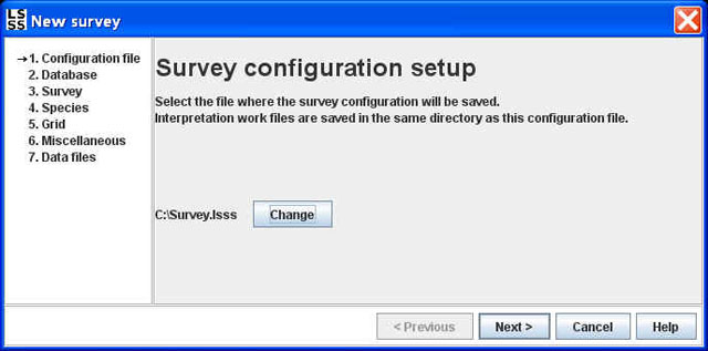
1) Choose survey.
In the "File" menu, choose "New Survey".
Then the survey configuration setup will pop up and guide the user through the entire setup.
A marker to the left in this window shows how far the setup has progressed.
During setup, the user can set a wide range of parameters related to storage of survey data and interpretation data.
In the setup, the user also selects the species that may be encountered in the interpretation session
(the list of species can also be updated at a later stage in the interpretation session).
The species can be chosen from a predefined list of about 3000 known marine species available in a table in LSSS.
Alternatively, the user can load an existing survey by choosing "Open Survey" under the File menu.
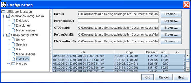
2) Select data.
The "Data files" window shown below will either pop up during setup of a new survey,
or it will pop up after an existing survey has been opened.
This window shows the files available in the chosen survey, and the user can then select all data files, or a subset.
3) If necessary, remove spikes and other types of noise.
4) Perform interpretation by using one or both of the following two methods.
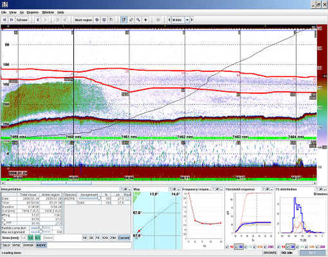
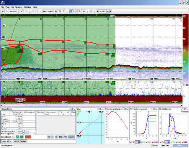
A) If the data contains wide layered species, such as different forms of plankton,
then start interpretation by defining initial layering by means of straight lines.
Then adjust the shape of the straight lines to better reflect the shape of the layered structures.
Finally, assign one or several species identifiers and species percentages to each interpreted region.
The species identifiers and percentages are entered in the Interpretation window,
normally located in the lower left part of the LSSS main window.
An example of a layered region is shown below.
B) If the data contains schools, then start interpretation by drawing a square around each school. Alternatively read predetected school regions (suggestions). Then adjust the shape of each region to better reflect the shape of the school. In this process, the squares can be transformed into arbitrarily shaped convex or concave regions. Finally, assign one or several species identifiers and species percentages to each region. An example of a school region is shown below.
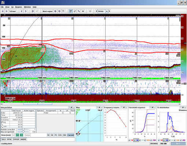
5) Save interpreted data and move to the next section to be interpreted in the echogram.
Saved interpretations will be marked with a green overlay as shown below.
The format of the interpreted data is described under the heading "Interpretation format".
6) If more data needs to be interpreted, then go to step 3 and repeat step 3,4,5
7) If needed, use the report generator to get an overview of the interpretation results.
8) Close survey.